


Authors:
(1) Mengshuo Jia, Department of Information Technology and Electrical Engineering, ETH Zürich, Physikstrasse 3, 8092, Zürich, Switzerland;
(2) Gabriela Hug, Department of Information Technology and Electrical Engineering, ETH Zürich, Physikstrasse 3, 8092, Zürich, Switzerland;
(3) Ning Zhang, Department of Electrical Engineering, Tsinghua University, Shuangqing Rd 30, 100084, Beijing, China;
(4) Zhaojian Wang, Department of Automation, Shanghai Jiao Tong University, Dongchuan Rd 800, 200240, Shanghai, China;
(5) Yi Wang, Department of Electrical and Electronic Engineering, The University of Hong Kong, Pok Fu Lam, Hong Kong, China;
(6) Chongqing Kang, Department of Electrical Engineering, Tsinghua University, Shuangqing Rd 30, 100084, Beijing, China.
Table of Links
2. Evaluated Methods
3. Review of Existing Experiments
4. Generalizability and Applicability Evaluations and 4.1. Predictor and Response Generalizability
4.2. Applicability to Cases with Multicollinearity and 4.3. Zero Predictor Applicability
4.4. Constant Predictor Applicability and 4.5. Normalization Applicability
5. Numerical Evaluations and 5.1. Experiment Settings
5.2. Evaluation Overview
We assess the methods using the previously described 16 test cases — for each test case, the methods are ranked according to the active branch flow accuracy and separately according to the nodal voltage accuracy, resulting in 32 linearization rankings[4]. To save space, we present here only four of these 32 rankings as representative examples. These rankings, illustrated in Figs. 2 to 5, cover various grid types, fluctuation levels, and data conditions, and will be discussed in subsequent sections. The other 28 evaulations are included in the supplementary material [55]. Additionally, to concisely represent the comprehensive accuracy ranking information, we summarize all the accuracy results into Figs. 6 and 7, respectively. The following accuracy analyses are largely drawn from these two figures. Lastly, Figure 8 presents the computational efficiency for all evaluated methods.
Remark: The evaluation outcomes of various methods are influenced by method configurations (e.g., hyperparameters) and/or the settings of test cases (e.g., whether the dataset contains constant predictors such as the voltages of PV nodes). Given this, we intend not to argue that one method is universally superior/worse in accuracy or computational efficiency than others. Rather, our analysis below focuses on identifying and analyzing notable and consistent outcomes from numerous tests across various methods, in terms of their accuracy, inaccuracy, under-performance, failure, excessive computation times, etc. In the meantime, we dive into the underlying reasons to provide a theoretical explanation for these notable and consistent phenomena, instead of merely showing simulation outcomes. This strategy, complemented by the use of cross-validation for tuning parameters, may help to reduce the impact of method configurations and/or test case settings on the evaluation results. Nevertheless, it is important to acknowledge that such an impact can never be fully eliminated.
5.3. Failure Evaluation
The figures below illustrate that certain evaluated methods encounter failures, which can be categorized into three distinct types:
• INA Type: Certain methods cannot calculate specific responses due to limitations in response selection generalizability, leading to inapplicability (INA) failures. For example, the PTDF method cannot determine unknown voltages, leading to its failure when voltages serve as the evaluation benchmark.
• NaN Type: Some methods cannot produce a complete numerical coefficient matrix for the linear model, instead containing NaN values[5], leading to NaN failures. This issue typically arises from attempts to invert a singular matrix during the training phase of a specific DPFL approach.
• OOT Type: Certain methods encounter computational limitations, leading to out-of-tolerance (OOT) failures. These limitations include exceeding the testing environment’s available RAM (16 GB in our study), surpassing MATLAB’s maximum array size (approximately 281.47 trillion elements in our study), or failing to complete training within a reasonable timeframe (set at one hour in our study). Such OOT failures underscore the significantly low computational efficiency of some approaches, especially optimization-based methods, when applied to larger test systems.

![⋄: Noise/outliers are only added to the training dataset; the testing data remains unpolluted; noise refers to the white Gaussian noise.‡: Within the training dataset’s matrix, columns represent various variables, both known and unknown, while rows are indicative of distinct samples. The term “Joint Noise” refers to a scenario where each element within a row is subjected to an identical noise level of 45dB, a level suggested by [54]. This implies that the entire system’s data were measured by a single device at any given time instance, a premise that may not align with real-world practices. The inclusion of this scenario serves not only to illustrate that “Joint Noise” does not significantly impact the training performance (as shown later), but also to encourage researchers to clearly specify their methods of introducing noise into the dataset.](https://hackernoon.imgix.net/images/fWZa4tUiBGemnqQfBGgCPf9594N2-gu9346a.png?auto=format&fit=max&w=3840)
In Figs. 6 and 7, failures are explicitly identified and labeled. The following provides detailed explanations for these failures.
INA-type Failure
First, For the calculation of active branch flows, methods LCP_BOXN, LCP_BOX, TAY (derived from the equations of nodal power injections in polar coordinates), LCP_JGDN, and LCP_JGD are not applicable, as discussed in Section 4.1 and identified in Table 3.
Additionally, for the calculation of nodal voltages, methods PTDF, LCP_COUN, and LCP_COU are not applicable, as explained in Section 4.1 and emphasized in Table 3.
NaN-type Failure
First, the methods LS, LS_CLS, and LS_REC frequently face NaN-type failures due to their inability to address the singularity issue arising from multicollinearity. However, in some test cases where multicollinearity is less evident, these methods may not encounter such failures.
Second, the PLS_BDLY2 method, which incorporates the active power injection at the slack bus into the predictor


dataset, experiences a more severe multicollinearity issue compared to PLS_BDL, as discussed in [6]. Consequently, PLS_BDLY2 may face NaN-type failures in certain scenarios where PLS_BDL does not. This also showcases the effectiveness of moving the active power injection at the slack bus to the response dataset.
Third, the failure of the PLS_RECW method is primarily attributed to NIPALS algorithm used for component extraction and data decomposition for PLS_RECW. Specifically, the issue arises when the predictor dataset’s loading and weight matrices, produced by the NIPALS algorithm, exhibit linear dependency among their columns. This dependency results in a singular matrix upon their multiplication. Consequently, the linear model’s coefficient matrix, derived from the inverse of this singular matrix, is rendered undefined, leading all coefficients to assume NaN values. A key underlying cause of this issue, especially when considering the successful performance of PLS_REC and PLS_NIP, is the implementation of the forgetting factor. In this study, a forgetting factor of 0.6, as referenced in [20], is applied. This factor effectively diminishes the influence of older samples due to its multiplication effect, as detailed in [6]. This mechanism is likely at the core of the observed numerical instability, as the failure issue of the PLS_RECW method is resolved when the forgetting factor is adjusted to 0.9.
OOT-type Failure
First, methods DRC_XYM and DRC_XM, both momentbased, employ conic dual transformation to convert constraints into equivalent semi-definite constraints. Given the high computational demand of semi-definite programming, it is no surprise that these methods begin to exceed the RAM capacity of the testing device at a system size of 118 buses.
Second, methods LS_LIFX and LS_LIFXi utilize dimension lifting, significantly increasing the dataset size with the test case scale. At a system size of 1354 buses, the dimension-lifted dataset surpasses MATLAB’s maximum array element limit.
Third, a range of methods, including LS_HBLD, LS_HBLE, LS_WEI, SVR, SVR_CCP, SVR_RR, LCP_BOX, LCP_BOXN, LCP_COU, LCP_COUN, LCP_JGD, LCP_JGDN, and DRC_XYD, either apply optimization-based approaches or use regression models but are solved via optimization programming. The number of decision variables (i.e., coefficient matrix elements of the linear model) exponentially increases with system size, rendering these methods unsolvable by commercial solvers at a system size of 1354 buses due to RAM constraints.
Lastly, methods SVR_POL and LS_GEN experience significant slowdowns at a system size of 1354 buses. The former is affected by its 3rd-order polynomial-kernel-based fitting process, while the latter’s iterative process and the use of pseudoinverse result in substantial time consumption when dealing with large matrices.
This paper is available on arxiv under CC BY-NC-ND 4.0 Deed (Attribution-Noncommercial-Noderivs 4.0 International) license.
[5] NaN means “not a number”. It occurs in case of undefined numeric results, such as 0 ÷ 0, 0 × ∞, ∞ ÷ ∞, etc.