How Different Sampling Strategies Affect Clustering Accuracy

Table of Links

Abstract and 1 Introduction

2 Preliminaries and Related Work

2.1 On Sampling Strategies

2.2 Other Coreset Strategies

2.3 Coresets for Database Applications

2.4 Quadtree Embeddings

3 Fast-Coresets

4 Reducing the Impact of the Spread

4.1 Computing a crude upper-bound

4.2 From Approximate Solution to Reduced Spread

5 Fast Compression in Practice

5.1 Goal and Scope of the Empirical Analysis

5.2 Experimental Setup

5.3 Evaluating Sampling Strategies

5.4 Streaming Setting and 5.5 Takeaways

6 Conclusion

7 Acknowledgements

8 Proofs, Pseudo-Code, and Extensions and 8.1 Proof of Corollary 3.2

8.2 Reduction of k-means to k-median

8.3 Estimation of the Optimal Cost in a Tree

8.4 Extensions to Algorithm 1

References

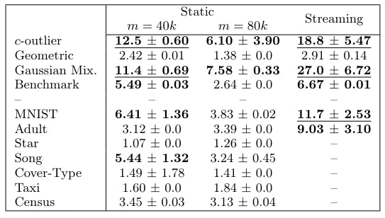
5.2 Experimental Setup

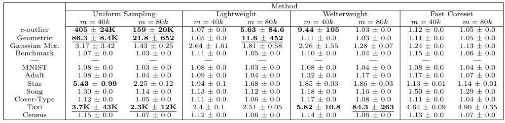
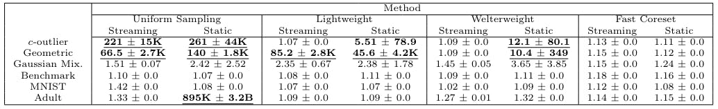
Algorithms We compare Fast-Coresets (Algorithm 1) against 4 different benchmark sampling strategies that span the space between optimal time and optimal accuracy, as well as state-of-the-art competitors BICO [38] and Streamkm++[1].

- Standard uniform sampling. Each point is sampled with equal probability and weights are set to n/m, where m is the size of the sample.

- Lightweight coresets [6]. Obtain a coreset by sampling sensitivity values with respect to the 1-means solution, i.e. sensitivities are given by sˆ(p) = 1/|P|+cost(p, µ)/ cost(P, µ), where µ is the dataset mean.

- Standard sensitivity sampling [47]. We refer to Section 2.

- BICO [38]. Utilizes BIRCH [58] to produce a k-means coreset in a stream.

- Streamkm++ [1]. Uses k-means++ to create large coresets for the streaming k-means task.

We do not compare against group sampling [25] as it uses sensitivity sampling as a subroutine and is merely a preprocessing algorithm designed to facilitate the theoretical analysis. By the authors’ own admission, it should not be implemented.

We use j going forward to describe the number of centers in the candidate j-means solution. Thus, lightweight coresets have j = 1 while Fast-Coresets have j = k.

We take a moment here to motivate the welterweight coreset algorithm. Consider that lightweight coresets use the 1-means solution to obtain the sensitivities that dictate the sampling distribution whereas sensitivity sampling uses the full k-means solution. In effect, as we change the value of j, the cluster sizes |Cp| in our approximate solution change. Referring back to equation 1, one can see that setting j between 1 and k acts as an interpolation between uniform and sensitivity sampling. We default to j = log k unless stated otherwise. We use the term ‘accelerated sampling methods’ when referring to uniform, lightweight and welterweight coresets as a group.

Datasets. We complement our suite of real datasets with the following artificial datasets. We default to n = 50 000 and d = 50 unless stated otherwise.

- c-outlier. Place n − c points in a single location and c points a large distance away.

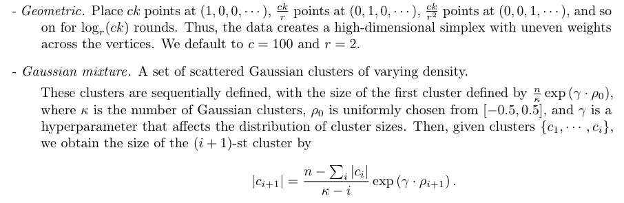
This has the property that all clusters have size n/k when γ = 0 and, as γ grows, the cluster sizes diverge at an exponential rate. We note that this is a well-cluster able instance with respect to cost stability conditions, see [3, 22, 46, 54].

The artificial datasets are constructed to emphasize strengths and weaknesses of the various sampling schemas. For example, the c-outlier problem contains very little information and, as such, should be simple for any sampling strategy that builds a reasonable representation of its input. The geometric dataset then increases the difficulty by having more regions of interest that must be sampled. The Gaussian mixture dataset is harder still, as it incorporates uneven inter-cluster distances and inconsistent cluster sizes. Lastly, the benchmark dataset is devised to be a worst-case example for sensitivity sampling.

Data Parameters In all real and artificial datasets, we add random uniform noise η with 0 ≤ ηi ≤ 0.001 in each dimension in order to make all points unique. Unless specifically varying these parameters, we default all algorithms in 5.2 to k = 100 for the Adult, MNIST, Star, and artificial datasets and k = 500 for the Song, Cover Type, Taxi, and Census datasets. Our default coreset size is then m = 40k. We refer to the coreset size scalar (the “40” in the previous sentence) as the m-scalar. We only run the dimension-reduction step on the MNIST dataset, as the remaining datasets already have sufficiently low dimensionality. We run our experiments on an Intel Core i9 10940X 3.3GHz 14-Core processor.